library(tidymodels)

# Compute the sample mean the tidymodels way:
point_estimate <- gss |>
    specify(response = hours) |>
    calculate(stat = "mean")

# Generate samples from the null distribution:
null_dist <- gss |>
    specify(response = hours) |>
    hypothesize(null = "point", mu = 40) |>
    generate(reps = 999, type = "bootstrap") |>
calculate(stat = "mean")tidymodels is a popular framework for regression, machine learning, and hypothesis testing. There’s been a lot of hype around it. There are courses focusing on tidymodels, and there are books about how to use it. I don’t use it myself: not in my own practice and not in my teaching. Here’s why.
Inconsistency in bootstrapping
My first issue with tidymodels is how it handles bootstrap methods. When bootstrapping using tidymodels, the results obtained using the standard methods for confidence intervals and p-values can differ. You can end up with a p-value that suggests significance while the confidence interval includes the null (or vice-versa).
To illustrate the problem, I’ll use the same dataset (gss) and the same null hypothesis as in the the official tidymodels documentation on how to perform hypothesis testing and compute confidence intervals. I use an example identical to that the tidymodels team uses in order to highlight that this isn’t just an issue that arises in pathological or cherry-picked examples. Quite the opposite: it’s something that is likely to arise any time that the p-value is close to the significance level of the test.
The data comes from the General Social Survey. Each row is an individual survey response. The null hypothesis is that the mean number of hours worked per week \(\mu\) in the population is 40, i.e., that \(\mu=40\)
First, we compute the mean, specify the null hypothesis and create bootstrap samples:
We can now run a two-sided test of \(H_0: \mu = 40\) (recall that the null hypothesis was specified in the previous step):
null_dist |> get_p_value(obs_stat = point_estimate,
                         direction = "two_sided")
# A tibble: 1 × 1
p_value
<dbl>
1 0.0400The p-value is 0.04: less than 0.05, and so at the 5% significance level we conclude that \(\mu \neq 40\).
Now, let’s compute a 95% confidence interval for \(\mu\):
null_dist |> get_confidence_interval(point_estimate = point_estimate,
                                     level = 0.95)
# A tibble: 1 × 2
lower_ci upper_ci
<dbl> <dbl>
1 38.7 41.3Uh-oh! This time, the conclusion is that \(\mu\) is somewhere between 38.7 and 41.3, which means that it could be 40. The conclusions from the test and the confidence interval differ.
tidymodels offers three different ways of computing bootstrap confidence intervals, none of which are consistent with the method it uses to compute bootstrap p-values. This can cause strange discrepancies whenever the p-value is close to the significance level (0.05 in this case).
In addition to the default percentile method shown above, the other methods available are referred to as the standard error method and bias-corrected intervals. These aren’t really the best bootstrap intervals available. The standard error method naively uses quantiles from the normal distribution when computing the confidence bounds. The bias-corrected interval is a simplified version of the celebrated BCa interval, that lacks the acceleration adjustment found in true BCa intervals, sacrificing the theoretical properties that justify its use.
To see that neither of these are consistent with the p-value, here’s an example from another run:
null_dist <- gss |>
    specify(response = hours) |>
    hypothesize(null = "point", mu = 40) |>
    generate(reps = 99, type = "bootstrap") |>
    calculate(stat = "mean")

null_dist |> get_p_value(obs_stat = point_estimate,
                         direction = "two_sided")
# A tibble: 1 × 1
p_value
<dbl>
1 0.0606This time, the p-value is greater than 0.05, so at the 5% level we’d say that we don’t have any statistical evidence that \(\mu\neq 40\). But \(\mu=40\) is not contained in the standard error method and bias-corrected confidence intervals, which would indicate that we actually do have evidence against the null hypothesis:
null_dist |> get_confidence_interval(point_estimate = point_estimate,
                                     level = 0.95,
                                     type = "se")
# A tibble: 1 × 2
lower_ci upper_ci
<dbl> <dbl>
1 40.1 42.7null_dist |> get_confidence_interval(point_estimate = point_estimate,
level = 0.95,
type = "bias-corrected")# A tibble: 1 × 2
lower_ci upper_ci
<dbl> <dbl>
1 41.2 42.1Confidence intervals and hypothesis tests are just two sides of the same coin, and if you’re doing things right, they should always be in agreement (mathematical details can be found here). Using a framework that allows the results from these to drift apart makes for confusing results and shaky inferences. Consistency is key, and tidymodels doesn’t give its users that.
What to use instead
As the package author, I’m heavily biased, but I think that boot.pval does a much better job here. It is designed to ensure that p-values are derived from the bootstrap distribution in a way that is mathematically aligned with confidence intervals, treating the bootstrap as a cohesive inferential tool rather than a collection of disconnected summary statistics. With boot.pval, the p-value will be less than \(\alpha\) if and only if the parameter is outside the corresponding \(1-\alpha\) confidence interval. boot.pval can be used for a wide range of problems, including tests for location, (generalised) linear models, survival models, and mixed models.
Plus, the code is much shorter too. To run a two-sided test of \(H_0: \mu = 40\), we only need a single line of code:
library(boot.pval)
boot_t_test(gss$hours, mu = 40)
    One Sample Bootstrap t-test (studentized)

data:  gss$hours
t = 2.0852, R = 9999, p-value = 0.0341
alternative hypothesis: true mean is not equal to 40
95 percent confidence interval:
 40.09744 42.72521
sample estimates:
mean of x
   41.382
But the tidymodels approach works, right?
Come on, I hear you say, why are you being such a pedant? The tidymodels approach to p-values works. You’re getting yourself worked up about silly details.
Well. Let’s consider the one-sample test about a mean from the previous section. The reason for using the bootstrap here instead of a classic t-test is that we then don’t have to worry about having a normal distribution for our data: the bootstrap should ensure that the test works even without normality.
Expect that not all bootstrap methods do. Good bootstrap methods, typically based on pivots, achieve second-order correctness, meaning that they often will do a much better job of computing correct confidence intervals or p-values than a traditional t-test1.
So what about the tidymodels bootstrap test?

I wanted to know how well the tidymodels bootstrap test for the mean performed compared to similar tests: a traditional normality-based t-test, a second-order correct studentised t-test from boot.pval (the default in that package), and a first-order correct percentile t-test from boot.pval. To find out, I ran simulations where the data came from different non-normal distributions, to see if the different tests had the correct type I error rate for non-normal data. I tried four different skew and bimodal distributions, shown below.
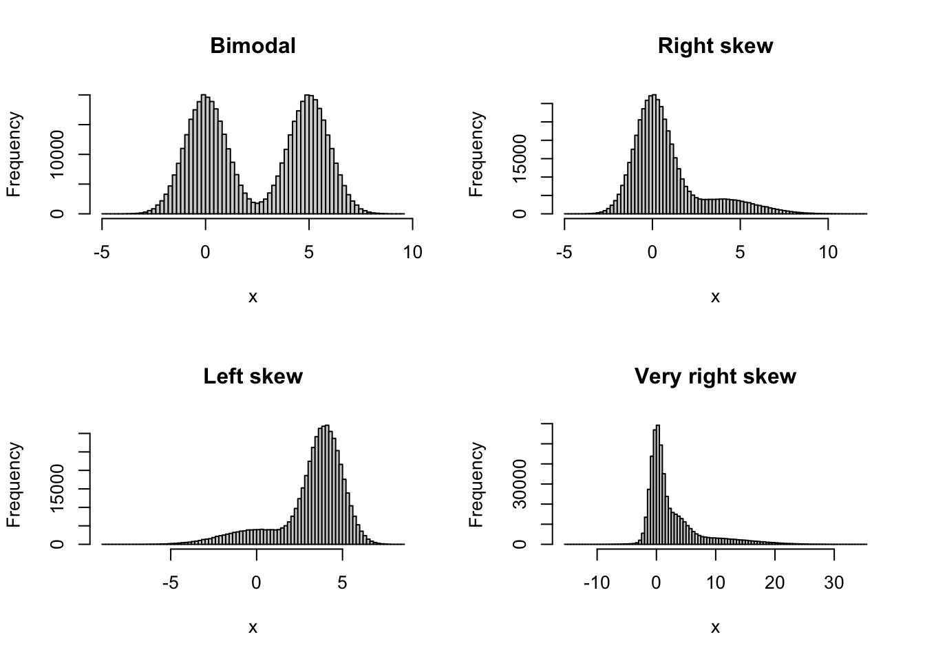
These are just the kind of situations where we might want to use the bootstrap. For each distribution, I simulated 100,000 samples under the null hypothesis. For each of these, I then ran the tests at the 5% significance level, and checked for how many runs each test yielded a significant result. The closer this proportion is to 0.05, the better the test performs in terms of the type I error rate. Here are the results for different combinations of distributions and sample sizes:
| Sample size | t-test | tidymodels test | boot.pval studentised test | boot.pval percentile test |
|---|---|---|---|---|
| Bimodal, n=25 | 0.0517 | 0.0828 | 0.0394 | 0.0696 |
| Bimodal, n=50 | 0.0508 | 0.06934 | 0.0502 | 0.0640 |
| Right-skew, n = 25 | 0.0700 | 0.1012 | 0.0656 | 0.0885 |
| Right-skew, n = 50 | 0.0602 | 0.0812 | 0.0577 | 0.0721 |
| Left-skew, n = 25 | 0.0681 | 0.0998 | 0.0639 | 0.0869 |
| Left-skew, n = 50 | 0.0587 | 0.0793 | 0.0560 | 0.0718 |
| Very right-skew, n = 25 | 0.0850 | 0.1240 | 0.0639 | 0.0980 |
| Very right-skew, n = 50 | 0.0682 | 0.0936 | 0.0552 | 0.0784 |
None of the tests perform perfectly. But the tidymodels test actually always performs worse than a regular t-test here! For the right-skew distribution with n=25 for instance, the tidymodels test performs like a test at the 10% level when we run it at the 5% level, rejecting 10% of all correct null hypotheses. In contrast, the studentised bootstrap t-test from the boot.pval package (shown in an example in a previous section) outperforms the traditional t-test in all scenarios except one (bimodal, n = 25).
In summary, bootstrap p-values and confidence intervals computed using tidymodels are not in agreement, which leads to confusion. In addition, the bootstrap test for the mean described in the tidymodels documentation fails to attain the nominal significance level. When you think that you run a test at 5% level, you might actually be running it at the 10% level.
This is my biggest criticism of tidymodels, but while I’m at it, let me mention a few other things that I don’t think make sense.
Missing feature: resampling regression models
I often want to bootstrap regression models. This can be done in several ways, the most common being residual resampling (where the model residuals are resampled) and case resampling (where the rows in the data are resampled). In the context of linear regression, residual resampling is often statistically superior to case resampling, particularly when predictors are fixed or maintaining the model’s structural integrity is paramount. Case resampling is better in some situations, for instance under heteroscedasticity.
While residual resampling has been a staple of the car package for decades, tidymodels restricts users to the case-resampling approach. Consequently, those who rely solely on tidymodels tutorials are left with the false impression that case resampling is the only way to bootstrap a regression, effectively narrowing their methodological toolkit. Which is silly, since residual resampling has a lot of merits, and has been around for a long, long time.
What to use instead
Despite offering a wider range of methods than tidymodels (including residual resampling), robust, long-standing packages like boot and car can feel dated to a new user compared to the pipe-friendly (well… more on that below) syntax of tidymodels. Indeed, the reason I created the boot.pval package, which effectively works as a wrapper for boot and (parts of) car, was to make the methods in those packages easier to use. Residual resampling of regression models can be done as follows:
library(boot.pval)
mtcars |>
    lm(mpg ~ hp + wt, data = _) |>
    boot_summary(method = "residual")
For case resampling, use method = "case" instead.
Again, let me stress that car and boot do all the heavy lifting here. But boot_summary makes it easy (I hope) to use these methods without having to write lots of code.
Missing feature: cross-validation
When it comes to resampling-based model evaluation, tidyverse misses Leave-One-Out Cross-Validation (LOOCV)2. While \(k\)-fold CV, available in tidymodels, is the darling of machine learning with large datasets, LOOCV remains a vital tool for smaller datasets where we need to minimise bias and randomness in our performance estimates. Indeed, many practitioners work with small-to-medium datasets where LOOCV is the gold standard. Not providing the method that best suits their need is an odd choice.
Why has LOOCV been left out? Well, in their Tidy Modeling with R book the tidymodels creators continue to perpetuate an old statistical myth regarding LOOCV’s performance, saying that it has poor statistical properties. When I wrote my book, I traced this misconception back to a 1983 paper by Bradley Efron. Efron made an unsubstantiated claim about LOOCV having poor properties, and this “fact” has been repeated for decades despite being repeatedly disproved.
By baking this misinformed opinion into the software’s design, tidymodels forces a specific (and flawed) view on its users. Since LOOCV is excluded from the core workflow, the framework implicitly signals that it isn’t important, steering users toward a one-size-fits-all approach to evaluation. Which, in this case, actually doesn’t fit all.
What to use instead
LOOCV is available in many packages, including tidymodels predecessor caret and the cv package. Here’s an example with cv:
library(cv)
mtcars |>
    lm(mpg ~ hp + wt, data = _) |>
    cv(k = "loo") |>
    summary()
n-Fold Cross Validation
method: hatvalues
criterion: mse
cross-validation criterion = 7.703321The pipe problem: a violation of R style
Then, there is the matter of syntax. The tidyverse philosophy is built on the power of the pipe (|>), where the logic is: Data |> Transform |> Model. This makes for clean code that is easy to read and write.
While tidymodels sometimes follows this logic, it also often inverts it. You frequently start a chain by defining a model specification or a recipe rather than starting with the data itself. Here’s what this can look like when we wish to run a linear regression:
lm_spec <- linear_reg() |> set_engine("lm")

model_fit <- workflow() |>
  add_model(lm_spec) |>
  add_formula(mpg ~ wt) |>
  fit(data = mtcars)
The data is an afterthought in the pipe chain, added at the very end. This breaks the flow that made pipes and the tidyverse intuitive in the first place. This isn’t just a nitpick; this way of writing code is genuinely bad R style that obscures the data-centric nature of R programming. If the syntax requires us to pipe backwards (starting with a model spec rather than the data), we are teaching beginners a mental model of R that is fundamentally at odds with the rest of the ecosystem. That’s just bad.
In addition, this is of course a terrible way to teach linear regression to beginners, as it buries the fundamental logic of linear regression under layers of unnecessary abstraction, ensuring that students learn the tidymodels framework rather than the statistics. I hope no one uses this for introductory statistics courses.
The Posit problem
It is impossible to discuss the modern R landscape without acknowledging the immense debt we owe to Posit. I’m writing this in RStudio and Quarto. I use the tidyverse every single day. These are amazing tools. Thank you, Posit.
However, this dominating position comes with a unique set of risks. Because Posit’s products historically have been of such high quality, many users, especially those new to the field, treat a Posit “recommendation” as an endorsement of scientific truth. Because Posit controls the IDE, the primary learning materials, and the most popular packages for R, a user can spend years in an Posit bubble without ever realising that there might be other ways of doing things. So if Posit builds a package like tidymodels and markets it heavily through their conferences, certifications, and documentation, it effectively becomes the “official” way to do statistics in R. It reshapes the community’s standards.
And problems then arise when the new standard is worse than other tools.
We must be careful not to confuse great software engineering with sound statistical guidance. Posit are great at the former, but the design of tidymodels shows that they aren’t infallible at the latter. Stay critical, and remember that just because a package has tidy in its name doesn’t mean it’s the best choice for your analyses.
Conclusion
A modelling framework should make good habits easy and bad habits hard. Unfortunately, tidymodels sometimes seems to do the opposite by omitting important tools. In the words of Sir David Cox, there are no routine statistical questions, only questionable statistical routines. tidymodels tries to offer solutions to the former, but often ends up with the latter.
I think you should stick with tools that prioritise statistical rigour over abstract workflows. I for one try to do just that. And that’s why I don’t use tidymodels.
Footnotes
To be a bit more precise, second-order correctness is related to the asymptotic performance of a method.↩︎
This is not strictly speaking true: the
rsamplepackage actually contains a method for LOOCV, but I can’t be used together with the functions used to evaluate predictive models in the othertidymodelspackages.↩︎